Model Diagnostics

Box-Cox

ravix.box_cox(model)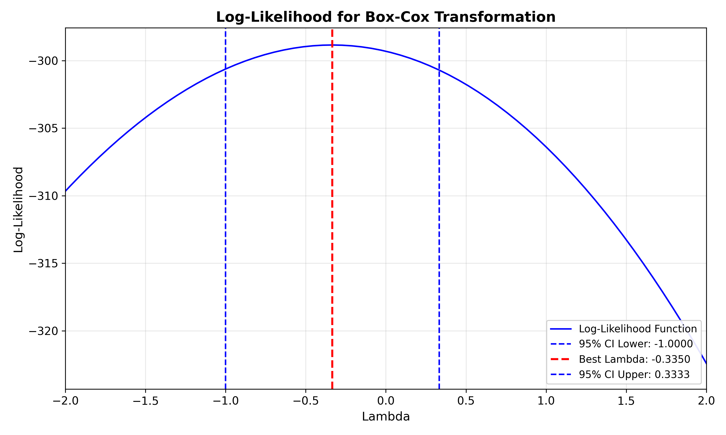

Heteroscedasticity — ravix.bp() and ravix.ncv()

Two complementary tests for non-constant residual variance. bp() runs the Modified Breusch-Pagan test; ncv() runs the Cook-Weisberg score test.

ravix.bp(model)

Breusch-Pagan Test for Heteroscedasticity
=======================================================
Test Statistic      : 1.1226
p-value             : 0.7716
Result              : Homoscedastic (p >= 0.05)
=======================================================

ravix.ncv(model)

Nonconstant Variance Test
=======================================================
Test Statistic      : 1.3498
p-value             : 0.2453
Result              : Constant variance (p >= 0.05)
=======================================================

Normality — ravix.shapiro()

ravix.shapiro(model)

Shapiro-Wilk Test for Normality
=======================================================
Test Statistic      : 0.9842
p-value             : 0.2769
Result              : Normal (p >= 0.05)
=======================================================

Residual histogram — ravix.hist()

ravix.hist(model)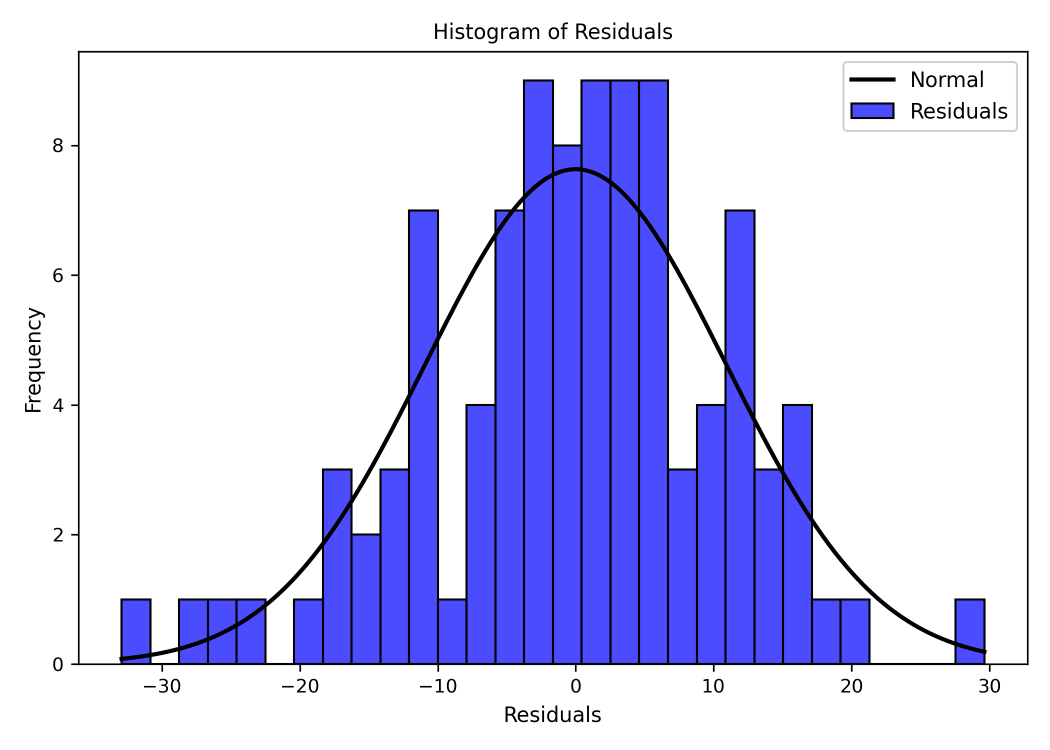

ravix.hist(model, norm = False, bins = 20)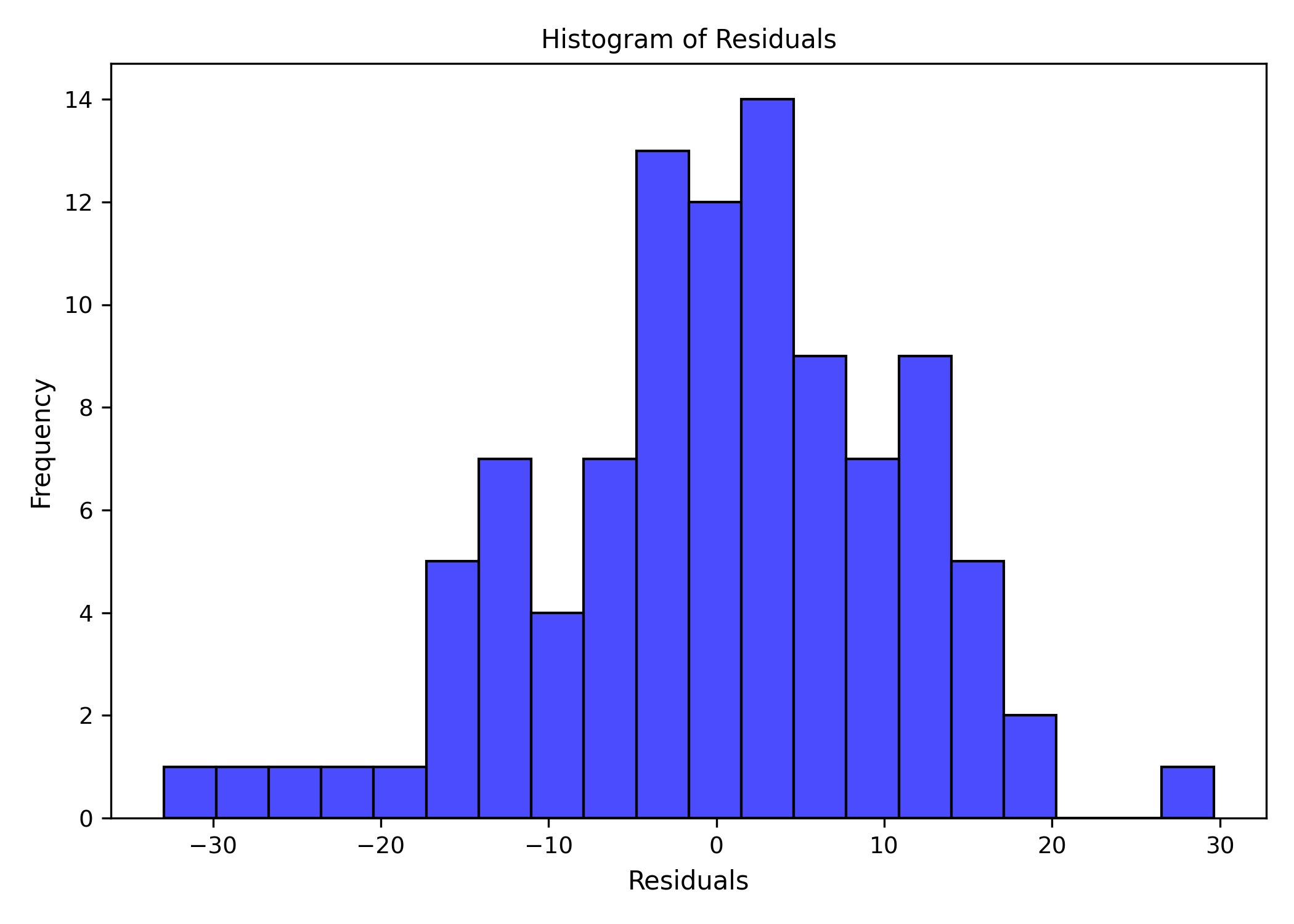

Variance Inflation Factors — ravix.vif()

Same call pattern as ravix.ols() — pass a formula and DataFrame directly.

ravix.vif("Price ~ .", df)

      TaxRate  Commercial    Income     Rooms
VIF  1.009601    1.059649  1.215393  1.268351

ravix.vif("Price ~ .", df, plot = True)

      TaxRate  Commercial    Income     Rooms
VIF  1.009601    1.059649  1.215393  1.268351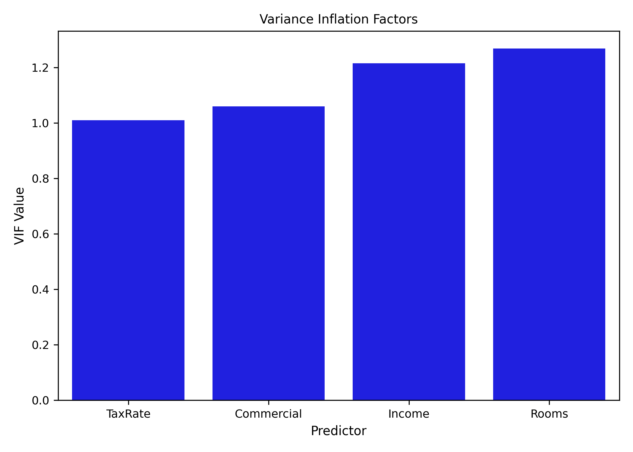

Q-Q plot — ravix.qq()

ravix.qq(model)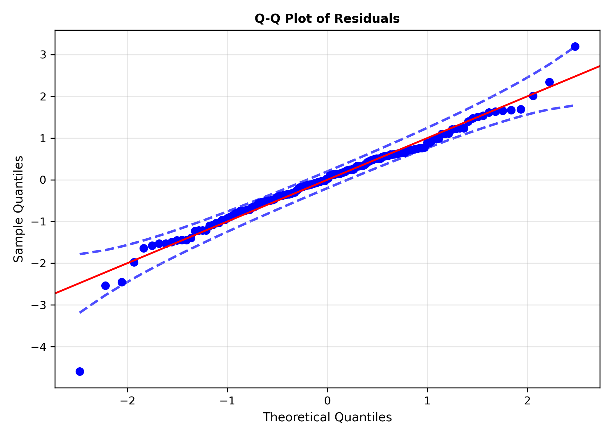

Cook’s distance — ravix.plot_cook()

ravix.plot_cook(model)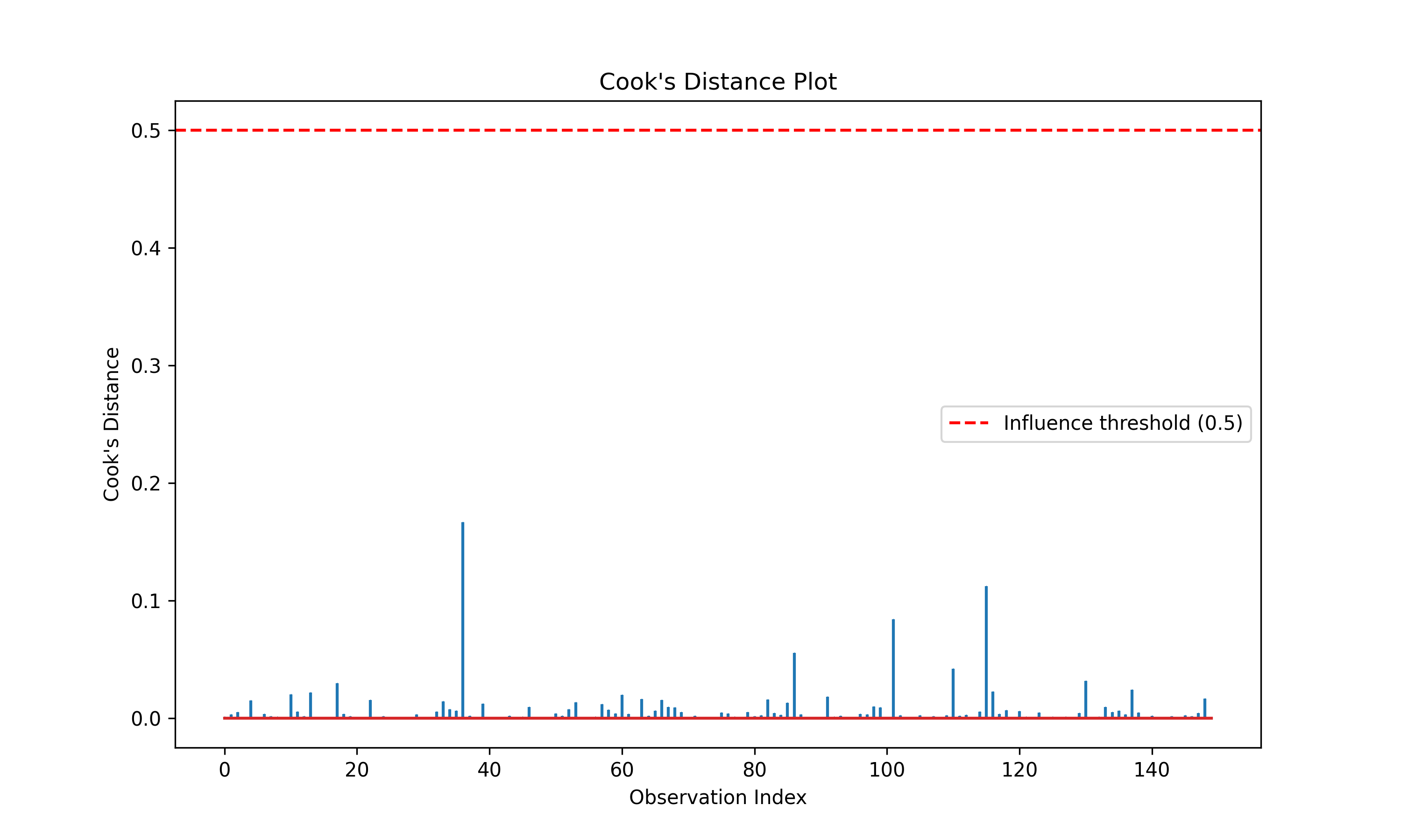

Textbook reference: Diagnostics are covered in Chapter 8 of Applied Linear Regression for Business Analytics with Python.